Real-Time Noise Floor Computer

Overview

In high school, I was lucky to be connected with Erik Johansson, an engineer working on the adaptive optics system on the Daniel K. Inouye Solar Telescope (DKIST). He helped me work on a senior year capstone project to take real data from DKIST and compute the noise floor in real time. This project was both my introduction to signal processing and also an interesting multithreaded challenge to synchronize regular arrival of dataframes with periodic, large calculations of the system noise floor. It was also a chance to learn how to write code that fit into a bigger system, as it had to accept actual processed signals from the lenslet array of an adaptive optics wavefront sensor.

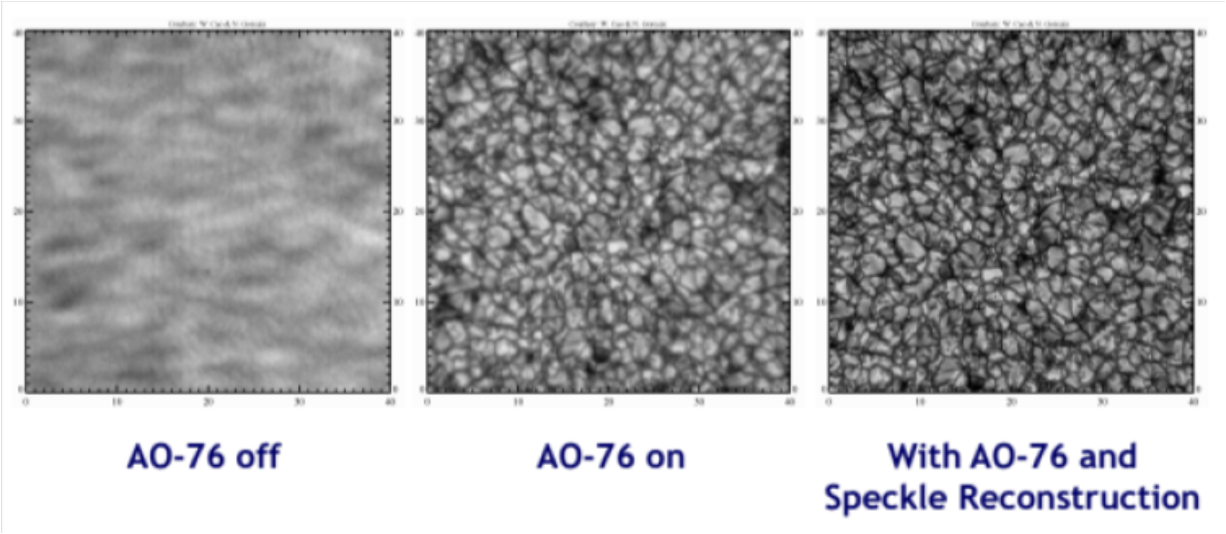
Three images of solar granulation: blurry with AO-76 off, sharp with AO-76 on, and sharper still with AO-76 plus speckle reconstruction — An image used to explain to me how the adaptive optics system on DKIST is able to clean up images of the sun.

How it works

Incoming data is split into overlapping segments (for example, length 300 with 50% overlap), and each segment has its mean removed.
A windowed periodogram is computed for each segment, with a Hamming window by default to reduce spectral leakage.
The periodograms are averaged, and the noise floor is estimated from the asymptote of the spectrum, then integrated and square-rooted to give an RMS value.
The heavy computation runs on a separate thread connected by queues, so data collection doesn’t stall (which would miss samples).

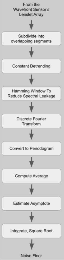
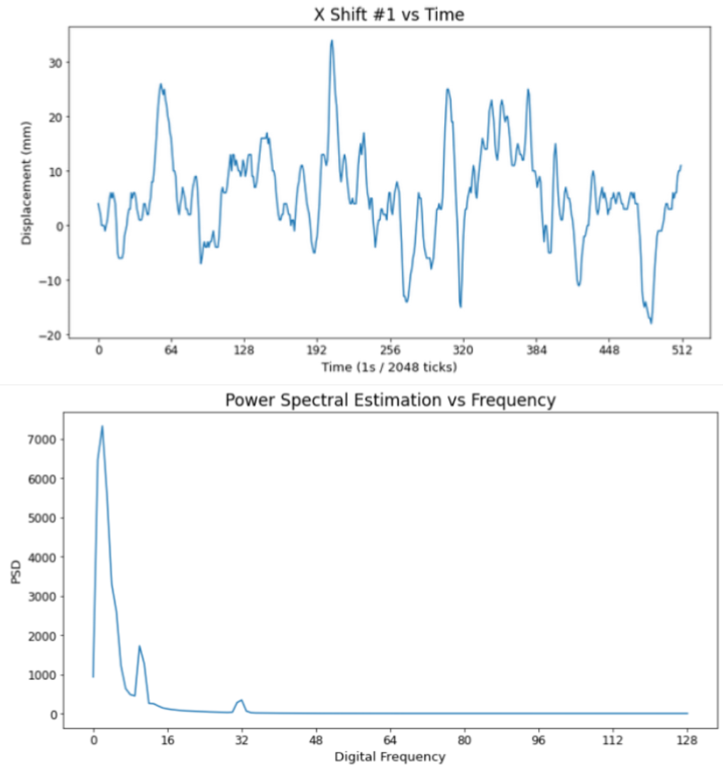
Flowchart: wavefront sensor lenslet array, subdivide into overlapping segments, constant detrending, Hamming window, discrete Fourier transform, convert to periodogram, compute average, estimate asymptote, integrate and square root, noise floor

Top: X shift of one lenslet over 512 samples, fluctuating between about -18 and 34 mm. Bottom: its averaged power spectral density, with a large peak near zero frequency, smaller peaks near 10 and 32, and a flat floor beyond

Left: the pipeline I built, from data collection to the noise floor. Right: an example output for one lenslet, its position over time (top) and averaged power spectrum (bottom).

Results

The above figure shows an example output from my system, both showing the low frequency atmospheric noise and the high frequency noise floor of the sample. The full system would report this noise floor over time.

I was really proud of this project when I finished it! The interface was clean, and the code was really fast. In retrospect, if I revisited it, I could get the same results in a few days instead of a few months, but some of these early projects in my career really taught me how fascinating engineering could be, and having a strong basis in signal processing allowed me to do better things in the future.